Watch or read?
Would you like to explore this example through a short video or text? If you prefer the video, check out the preview on the right (or below if you’re on a mobile device).
The video includes animated explanations and additional examples.
Prefer text? Just keep reading!
Introduction
“It’s not rocket science” or “It’s not nuclear physics”—people say this when they want to imply something isn’t complicated. But here’s the truth: Rocket science and nuclear physics were developed by ordinary humans, not superheroes. That means you can understand them too—and even work with them one day.
In this article, we’ll break down a real task nuclear engineers face and show how they use the same math, chemistry, and physics you’re learning right now in school.
Nuclear power
Nuclear fuel: 100,000× more efficient than coal
Nuclear power is incredibly efficient—over 100,000 times more efficient than coal. That means just 2.2 pounds (1 kg) of uranium fuel delivers the same energy as 220,000 pounds (100,000 kg) of coal! Plus, unlike coal, nuclear energy produces zero carbon emissions.
How nuclear plants generate electricity
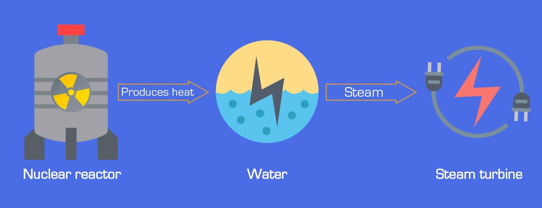
Nuclear plants turn heat into electricity in three steps:
- Nuclear reactions produce enormous heat.
- Heat boils water into high-pressure steam.
- Steam spins turbines to generate electricity.
Safety: the top priority
Nuclear plants follow the strictest safety rules because of radioactivity risks. Every component—from fuel rods to cooling systems—must be designed with extreme precision. That’s where math like integrals becomes critical (we’ll see how soon).
Integrals predicting corrosion in nuclear reactors
Corrosion in nuclear reactors
Over time, the metal parts inside a nuclear reactor corrode—meaning they oxidize (you might recognize this from chemistry lessons as redox reactions). This process causes the reactor’s components to gradually break down as they react with their environment.
Nuclear engineers need to predict exactly how long the reactor can operate safely, and the corrosion rate is one of the most critical factors in this calculation. It measures precisely how fast the metal deteriorates.
Mathematical function of the corrosion
Mathematical function
You’ve learned in math class that real-world processes can be described using mathematical functions. Corrosion is one such process. Here’s the actual function nuclear engineers use to predict reactor corrosion:
\( f(t) = 1.09 \times 10^{-2} \cdot t^{-0.65} \)
This function calculates:
What: Grams of stainless steel (the reactor material)
Where: Per square meter
When: Converted to oxide each second (units: g/(m²·s))
(All values use SI units – the international standard for nuclear power calculations.)
By integrating this function, we can predict exactly how reactor materials degrade over time. But first, let’s visualize it by plotting the graph.
Plotting the graph
Graph details:
- Function: f(t) = 1.09 times 10 to the negative 2, multiplied by t to the power of negative 0.65
- Trend: Corrosion rate decreases as time increases
- Interactivity: Press 'H' to hear coordinates. 'Ctrl/Cmd+F' opens accessibility settings.
This graph shows:
- x-axis: Time (seconds)
- y-axis: Corrosion rate (g/(m²·s))
Notice how the corrosion rate decreases every second—this matches our function’s behavior.
Calculating amount of corrosion graphically
To find total corrosion, we calculate the area under the curve between two time points. For example, between 1 and 2 seconds:
- Approximate the area as a trapezoid:
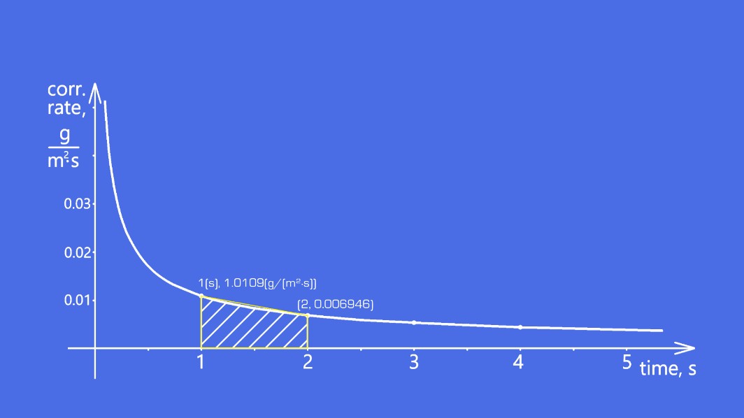
\[
\text{Area} = \frac{0.0109 + 0.006946}{2} \times 1 = 0.008923 \ \text{g/m}^2
\]
(This means ~0.008923 g of steel oxidizes per m² in that second.)
- Limitation:
While trapezoids work for short periods, they’re impractical for long timescales (e.g., a year = 31,536,000 seconds!). - Better tool:
Integrals give exact results with a single calculation—no approximation needed.
Calculating amount of corrosion using integral
Take another look at the graph above. Notice how the actual curve dips below our trapezoid estimate? Using a definite integral captures this exact shape, giving us a precise calculation. Let’s compute it for 1 to 2 seconds and compare with our earlier trapezoid estimate.
Antiderivative
First, we find the antiderivative of the corrosion function:
\[
\int 1.09 \times 10^{-2} \cdot t^{-0.65} \, dt = \frac{1.09 \times 10^{-2}}{0.35} \cdot t^{0.35} + C
\]
Definite integral
Now, evaluate from 1 to 2 seconds:
\[
\int_1^2 1.09 \times 10^{-2} \cdot t^{-0.65} \, dt = \left[ \frac{1.09 \times 10^{-2}}{0.35} \cdot t^{0.35} \right]_1^2 \approx 0.008551 \ \text{g/m}²
\]
Key comparison:
– Trapezoid estimate: 0.008923 g/m²
– Integral result: 0.008551 g/m²
The integral’s result (0.008551 g/m²) is slightly lower than the trapezoid’s estimate (0.008923 g/m²). Why? Because the actual corrosion curve dips below our straight-line approximation—and the integral accounts for this exact shape.
Want to see more? Watch the video!
The video version brings these concepts to life with:
Interactive animations of corrosion over time
Real-world examples, including:
1-year corrosion calculation (31,536,000 seconds!)
15-year projections used in actual reactor design
Visual comparisons between trapezoid and integral methods
Preview the video to see how integrals enable precise corrosion predictions in nuclear engineering.
Conclusion
Mathematics unlocks the hidden patterns of our world. From:
Nuclear engineering (corrosion rates in reactors)
Pharmaceutical research (drug concentration in blood)
Quantitative finance (dynamic investment models)
—these all often follow mathematical functions. By integrating these functions, we transform instantaneous changes into total quantities: exact material loss, precise dosage curves, or compounded returns.
The next time you see a curve, remember: beneath its shape lies a tool that powers science and industry—the integral.